The Phase Response Curve and its relevance for Neuroscience

The source for this post is mainly the book Dynamical Systems in Neuroscience by Eugene M. Izhikevich

We start considering a dynamical system that describes an oscillator of the form

dx/dt = f(x(t)) + Aδ(t - t_s), x ∈ R^m (1)

i. e. it admits an exponentially stable limit cycle and experiences pulse stimulation at times t_s, that istantaneously increase the state variable by amplitude A. We can imagine it as a periodically spiking neuron that experiences pulse stimulations at certain times. Many types of oscillators can be described by a single variable, i. e. the phase θ (for example in the case in which couplings are weak and effects on the amplitudes can be disregarded). The phase is usually taken as the time since the last spike, so the phase is taken equal to zero in correspondence of the peak of the spike. We say that a function x(t) is periodic if there is a costant T > 0 such that x(T + t) = x(t) for any t. The minimum value of T is called the period. Periodic functions appear in dynamical systems having limit cycle attractors. As t increases, past T, 2T, the phase variable wraps around the interval [0,T]. We can treat the interval [0,T] as a circle, where the θ variable is defined.

Consider a periodically spiking neuron (1) that receives a single brief pulse of current. Such a perturbation may change the timing of the spike, that is, the phase of the following spikes. The magnitude of the phase shift of the spike train depends on the exact timing of the stimulus relative to the phase of oscillation θ. Stimulating the neuron at different phases we can measure the phase response curve

PRC(θ) = θ_new - θ

Positive (negative) values of the function correspond to phase advances (delays) in the sense that they advance (delay) the timing of the next spike.

We want now to reduce the system described by eq. (1) to a phase model exploiting the phase response curve, following the method of Winfree (A. Winfree, 1967). We can actually be more general and consider a generic stimulation, i. e. not just described by a δ function but by a continuous function p(t).

dx/dt = f(x) + εp(t)

This equation describes a self sustained oscillator forced by a time-dependent input εp(t). ε is assumed to be sufficiently small that the trajectory of the weakly perturbed oscillator remains near the limit cycle attractor but greater than zero. If ε = 0 we can trasform dx/dt = f(x) to dθ/dt = 1, exploiting the fact that θ is defined in the interval [0,T] as θ = t. Now we are going to apply the same trasformation in the case in which ε ≠ 0.

Linear scaling of the PRC with respect to the strength of the pulse motivates the substitution PRC(θ,A) = AZ(θ), where Z(θ) is the linear response or sensitivity function, describing alteration of istantaneous frequency of oscillation after application of a small stimulus. It is informative to call it the infinitesimal PRC. Now let us substitute εp(t) with the equivalent train of pulses of strength A = εp(t_n)h where h is a small interpulse interval (the continuous function p(t) is approximated by an equivalent train of pulses of variable amplitudes).

We can write the corresponding Poincaré map, that relates the phase when pulse at time t_{n + 1} arrives (θ(t_{n + 1})) to the phase when the pulse at time t_n arrives (θ(t_n)) (one can verify indeed that θ(t_n+1) = (θ(t_n) + PRC(θ(t_n)) + T_s)mod T = (θ(t_new) + T_s)mod T for periodic stimulations with period T_s). The following Poincaré phase map thus holds:

θ(t_n+1) = (θ(t_n) + Z(θ(t_n))εp(t_n)h + h)mod T

hence, dividing by h and taking the limit for h that goes to 0, we obtain

dθ/dt = 1+ εZ(θ)p(t) (3)

We have so obtained a powerful reduction of the system of equation (1) or (2) to a phase model that exploits the Phase Response Curve, and that can predict the behavior of the oscillator to any kind of perturbation. The PRC gives important information on the synchronization properties of an oscillator, and depends on the bifurcations of the spiking limit cycle. For example, when the oscillations appear via saddle-node on invariant circle bifurcation the PRC has only positive values (Class 1 oscillator), while in the case of a supercritical Andronov-Hopf bifurcation it changes sign (Class 2 oscillator).

We can consider as an example the Morris Lecar Model, that, depending on the parameters’ values, behaves either as a Class I or a Class II oscillator.

The code to simulate such a model is below (where the package numba is used for computational ease), and where T0 is the observed period (in units of dt) between spikes.

# Morris Lecar model
# PRC of type II

import numpy as np
import matplotlib.pyplot as plt
from numba import njit

trials = 300
time = 500
dt = 0.001
N = int(time/dt)
C = 5
g_L = 2
V_l = -60
g_ca = 4
V_ca = 120
g_K = 8
V_K = -80 
phi = 1/15
V_1 = -1.2
V_2 = 18 
V_3 =4
V_4 = 17.4
I_ext = 45
T0 = 62612

times = []
currents = np.ones((trials,N))*I_ext
for s in range(trials):
    trand = np.random.randint(0,T0)
    currents[s,T0*3 + trand] = 3000
    times.append(T0*3 + trand)


@njit
def sim(T,dt,trials, currents):
    V = np.zeros((trials,int(T/dt)))
    N = np.zeros((trials,int(T/dt)))
    num = int(T/dt)
    for s in range(trials):
        for t in range(num - 1):
            M_inf = 1/2*(1 + np.tanh((V[s,t]-V_1)/V_2))
            N_inf = 1/2*(1 + np.tanh((V[s,t]-V_3)/V_4))
            tau = phi*np.cosh((V[s,t] - V_3)/(2*V_4))
            V[s,t+1] = V[s,t]  + (currents[s,t] -g_L*(V[s,t]-V_l) - g_ca*M_inf*(V[s,t]-V_ca) -  g_K*N[s,t]*(V[s,t]-V_K))*dt/C
            N[s,t + 1] = N[s,t] + tau*(N_inf -N[s,t])*dt
    return V,N
V,N = sim(time,dt,trials,currents)

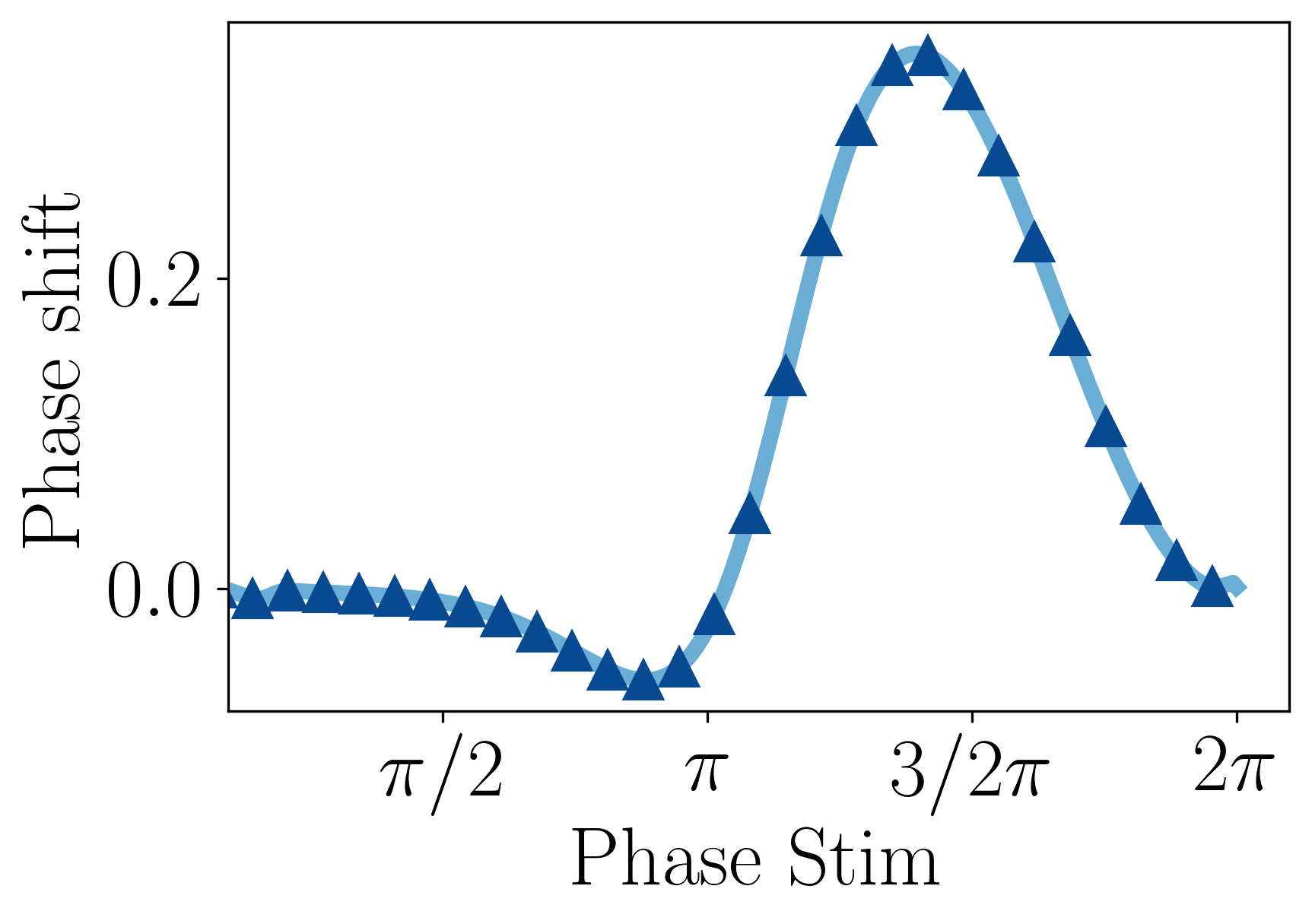
In order to get the PRC, in the above lines of codes the value of the external current is increased at random times in order to simulate istantaneous stimulations. After simulating the model, for each phase at which the stimulation arrives one studies the value of the induced phase shift. In this case the obtained phase response curve is this.

Since it has also negative values, it is a type II PRC.

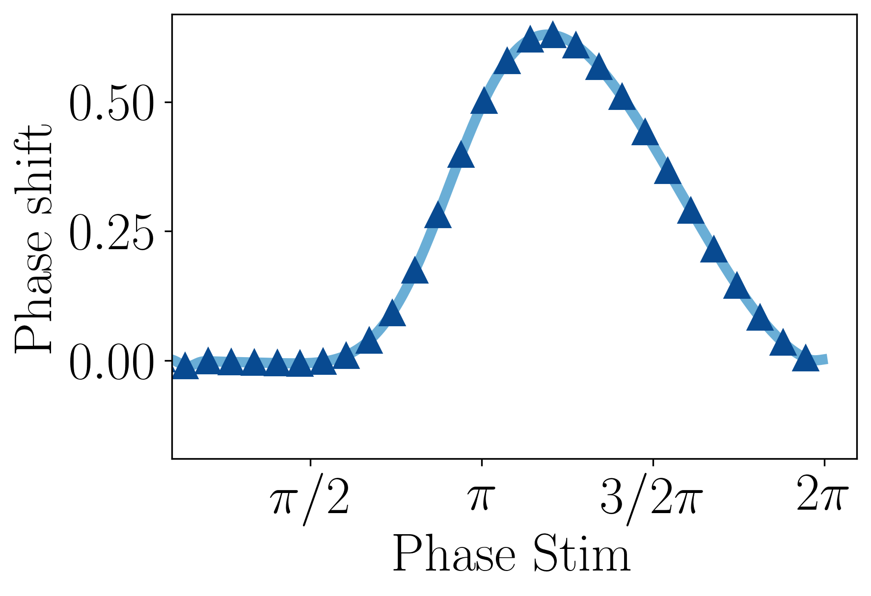
Changing the value of the parameter V₃ to 15 and I_ext to 39 (and, since changing the parameters affects the period, T0 is changed to the observed value, which is 106380 - in units of dt), the PRC now obtained is of type I.

Thus one could now model the Morris Lecar model with equation (3) and the obtained PRCs and predict its behavior to generic perturbation. Given the important implications and predictive power of the PRC, it is very promising to reconstruct it from data, as done here or here.